TICS-579-Deep Learning

Clase P1: Álgebra Tensorial

Alfonso Tobar-Arancibia

alfonso.tobar.a@edu.uai.cl

Introducción

Historia

La verdad podríamos estudiar historia e importancia de porqué el Deep Learning es importante, pero la verdad…

NO TENEMOS TIEMPO PARA ESO.

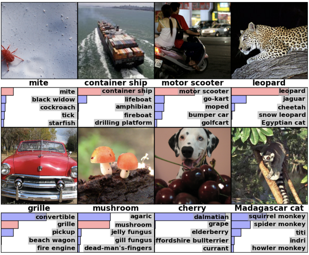
Alexnet (2012)

Transformers (2017)

GPT (2019)

LLMs (2023) (ChatGPT/Llama)

¿Por qué estudiar Deep Learning?

Imágen tomada de la Clase de Zico Colter

¿Por qué estudiar Deep Learning?

Facilidad y Autograd

• Frameworks como Tensorflow, Pytorch o Jax permiten realizar esto de manera mucho más sencilla.
  • Frameworks permiten calcular gradientes de manera automática.
  • Antigua mente trabajar en Torch, Caffe o Theano podía tomar cerca de 50K líneas de código.

Cómputo

• Proliferación de las GPUs, TPUs, HPUs, IPUs, como sistemas masivos de Cómputos.
  • How many computers to identify a cat? 16,000

Estado del Arte

• Modelos de Deep Learning pueden generar sistemas que entiendan imágenes, textos, audios, videos, grafos, etc.

Prerrequisitos

Tensores

Corresponde a una generalización de los vectores y matrices que permite representar datos de múltiples dimensiones.

Escalares (Orden 0)

\[-1, 11.27, \pi\]

Vectores Filas (Orden 1)

\[\begin{bmatrix}1.0 & -0.27 & -1.22\end{bmatrix}\]

Vectores Columnas (Orden 1)

\[\begin{bmatrix} 1 \\ -0.27\\ -1.22 \end{bmatrix}\]

Matrices (Orden 2)

\[\begin{bmatrix} 1.0 & -0.27 & 3\\ 3.15 & 2.02 & 1.2\\ -1.22& 0.55 & 3.97 \\ \end{bmatrix}\]

Normalmente los tensores utilizan un mismo tipo de dato: Integers o Float es lo más común.

Tensores

Tensores (Orden 3+)

\[\begin{bmatrix} \begin{bmatrix} 0.2 & 0.1 & -0.25 \\ 0.1 & -1.0 & 0.22\\ \end{bmatrix} \\ \begin{bmatrix} 0.24 & 0.1 & -0.25 \\ 0.05 & -0.69 & 0.98 \end{bmatrix} \\ \begin{bmatrix} 0.66& -1.0 & 0.22\\ -0.07 & -0.59 & 0.99 \end{bmatrix} \\ \begin{bmatrix} 0.16& 1.0 & 3.22\\ 9.17 & 7.19 & 9.99 \end{bmatrix} \end{bmatrix} \]

Nomenclatura

• \(\alpha\), \(\beta\), \(\gamma\): Minúsculas griegas denotan a Escalares.
• x, y, z: Minúsculas latinas denotan a Vectores.
• X, Y, Z: Mayúsculas latinas denotan a Matrices o Tensores.

Shape/Tamaño: Tamaño del tensor, tiene tantas dimensiones como su orden.

• Escalar: No tiene dimensiones.
• Vector: Tamaño es equivalente al número de elementos del vector. (3,)
  • A veces se usa la versión (1,3) para vectores filas y (3,1) para vectores columnas.
• Matrices: Tamaño es equivalente al número de filas y columnas. Ejemplo: (3,3)
• Tensores: Tamaño es equivalente al número de matrices que lo componen y el número de filas y columnas de cada una de ellas. Ejemplo: (4,2,3)

Importante

• La primera dimensión del shape se conoce como Batch Size el cual denota la cantidad de elementos de orden inferior.

• (3, ) tenemos 3 escalares.

• (3,2) tenemos 3 vectores filas de 2 elementos cada uno.

• (4,2,3) tenemos 4 matrices de (2,3) cada una.

Vectores: Suma

Corresponde a un arreglo unidimensional de números reales. Se puede representar como fila o columna. Por convención denotaremos \(\bar{x}\) como vector columna y \(\bar{x}^T\) como vector fila.

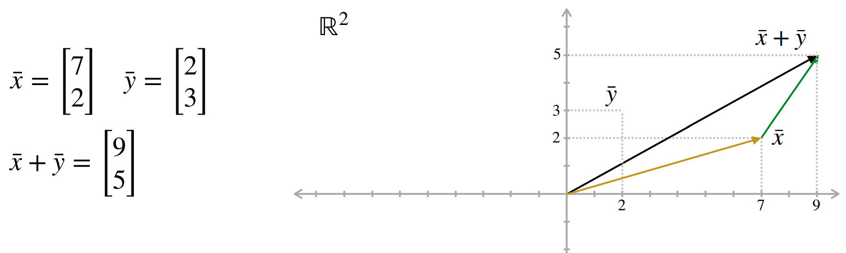
Operación Suma

• Permite sumar dos vectores de igual tamaño dimensión por dimensión.

Ej: \([7,2]^T + [2,3]^T = [9,5]^T\)

Propiedades

• Conmutatividad: \(\bar{x}+\bar{y} = \bar{y}+\bar{x}\)
• Asociatividad: \((\bar{x}+\bar{y})+\bar{z} = \bar{x}+(\bar{y}+\bar{z})\)
• Elemento Neutro: \(\bar{x} + \bar{0} = \bar{x}\)

Vectores: Ponderación

Corresponde a un arreglo unidimensional de números reales. Se puede representar como fila o columna. Por convención denotaremos \(\bar{x}\) como vector columna y \(\bar{x}^T\) como vector fila.

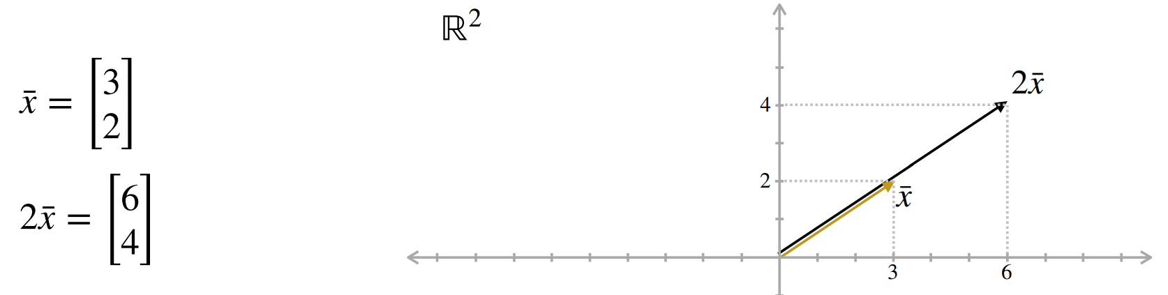
Operación Ponderación

• Permite multiplicar/ponderar cada dimensión del vector por un escalar.

  Ej: \(2 \cdot [3,2]^T = [6,4]^T\)

Propiedades

• Distributividad Escalar: \(a(\bar{x}+\bar{y}) = a\bar{x} + a\bar{y}\)
• Distributividad Vectorial: \((a+b)\bar{x} = a\bar{x} + b\bar{x}\)
• Elemento Neutro: \(1\cdot \bar{x} = \bar{x}\)
• Compatibilidad: \(a(b\bar{x}) = (ab)\bar{x}\)

Vectores: Norma

Norma (Euclideana)

Para un vector \(\bar{x}=[x_1, ..., x_n] \in \mathbb{R}^n\) se define la norma como:

\[||\bar{x}|| = \sqrt{\sum_{i=1}^n x_i^2}\]

Propiedades

• Desigualdad Triangular: \(||\bar{x}+\bar{y}|| \leq ||\bar{x}|| + ||\bar{y}||\)
• \(||\alpha \bar{x}||= |\alpha| \cdot ||\bar{x}||\)
• \(||\bar{x}|| = 0 \Longleftrightarrow \bar{0}\)

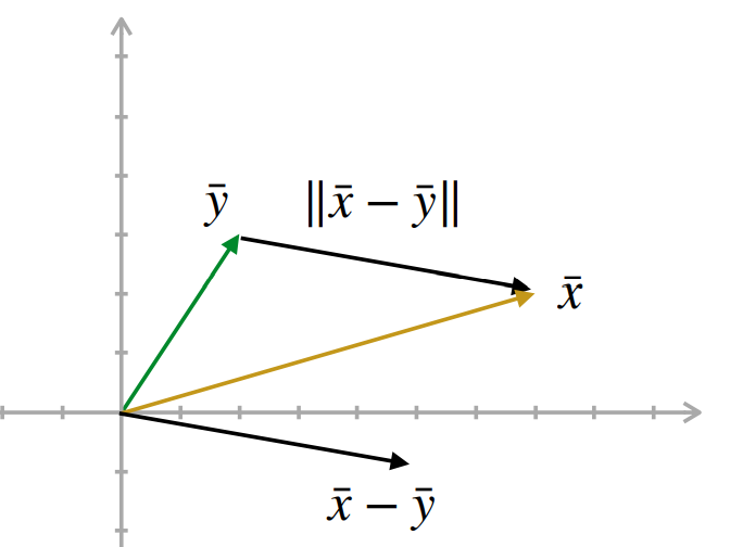
Aplicación

La norma permite calcular la distancia entre dos vectores.

\[d_{x,y} = ||\bar{x} - \bar{y}||\]

También serviría para puntos. ¿Por qué?

Vectores: Producto Interno (Producto Punto)

Inner Product or Dot Product

El producto interno entre dos vectores en \(\mathbb{R}^n\) se define como:

\(\bar{x} = [x_1, ..., x_n]\) e \(\bar{y} = [y_1, ..., y_n]\)

\[ \bar{x} \cdot \bar{y} = ||\bar{x}|| ||\bar{y}|| Cos\theta = \sum_{i=1}^n x_i y_i = x_1 y_1 + ... + x_n y_n\]

A veces el producto interno se denota como \(\bar{x}^T \bar{y}\) o \(\langle \bar{x}, \bar{y} \rangle\).

Propiedades

• Conmutatividad: \(\bar{x} \cdot \bar{y} = \bar{y} \cdot \bar{x}\)
• Linealidad: \((\alpha \bar{x})\cdot \bar{y} = \alpha(\bar{x}\cdot \bar{y})\)
• Distributividad: \(\bar{x} \cdot (\bar{y} + \bar{z}) = (\bar{x} \cdot \bar{y}) + (\bar{x} \cdot \bar{z})\)
• \(||\bar{x}||^2 = \bar{x} \cdot \bar{x}\)

Aplicaciones

• Ortogonalidad: Dos vectores son ortogonales si su producto interno es cero.
• Similaridad: Se puede usar el Cosine Similarity para calcular qué tan parecidos son dos vectores.

Cosine Similarity

\[sim(\bar{a}, \bar{b}) = \frac{\bar{a} \cdot \bar{b}}{||\bar{a}|| \cdot ||\bar{b}||}\]

• 1 implica misma dirección (idénticos)
• -1 implica direcciones opuestas (opuestos).
• 0 implica totalmente distintos (ortogonales).

Vectores: Otras Propiedades

Combinación Lineal

• Se denomina una combinación lineal de vectores a la suma ponderada de estos.

Ej: \(\bar{w} = \alpha \cdot \bar{x} + \beta \cdot \bar{y} + \gamma \cdot \bar{z}\)

\(\bar{w}\) es una combinación lineal de los vectores \(\bar{x}, \bar{y}, \bar{z}\).

Independencia Lineal

• Un conjunto de vectores es linealmente independiente si:

\(\alpha_1 \cdot \bar{x}_1 + \alpha_2 \cdot \bar{x}_2 + ... + \alpha_n \cdot \bar{x}_n = 0\) implica que \(\alpha_i = 0\) para todo \(i\).

👀 Ojito

Hay otras propiedades sumamente importantes de vectores, por lo que coloquen atención al curso de Algebra Lineal.

Matrices

Matrices: Definición

Corresponde a un arreglo bidimensional de números reales. Se dice que una matriz es de \(m\times n\) o que es \(\mathbb{R}^{m \times n}\) cuando tiene \(m\) filas y \(n\) columnas.

\[A = \begin{bmatrix} A_{1,1} & \dots & A_{1,n} \\ A_{2,1} & \dots & A_{2,n} \\ \vdots & \ddots & \vdots \\ A_{m, 1} & \dots & A_{m,n} \\ \end{bmatrix} \in \mathbb{R}^{m \times n}\]

👀

• Normalmente se utiliza \(m\) para denotar el número de registros y \(n\) como el número de features de un dataset tabular (o también conocido como Dataframe).
• Si \(m=n\) nos referimos a una matriz cuadrada.

Matrices: Notación

Si \(A\) es una matriz entonces:

• \(A_{i,j}\) corresponde al elemento en la fila \(i\) y columna \(j\). Es decir, un escalar.
• \(A_{i,:}\) corresponde a la fila \(i\) completa. Es decir, un vector fila.
• \(A_{:,j}\) corresponde a la columna \(j\) completa. Es decir un vector columna.

\[A = \begin{bmatrix} 0.2 & 1 & -5.2 & 3.1 & -1.3 \\ -0.5 & 10 & 0 & 3.1 & 3 \\ 2 & 25 & -5.2 & 0 & 0 \\ 100 & 3.4 & 4.1 & 0 & 42 \end{bmatrix}\]

Importante: Recordar que los índices en Python son 0-based.

• \(A_{2,4} = 3.1\)
• \(A_{:,3} = \begin{bmatrix}-5.2 & 0 & -5.2 & 4.1\end{bmatrix}^T\)
• \(A_{1,:} = \begin{bmatrix} 0.2, 1, -5.2, 3.1, -1.3\end{bmatrix}\)

Matrices: Suma

Operación Suma

• Permite sumar dos matrices elemento a elemento.

  Ej: Sea \(A\) y \(B\) dos matrices:

\[A = \begin{bmatrix} A_{1,1} & \dots & A_{1,n} \\ A_{2,1} & \dots & A_{2,n} \\ \vdots & \ddots & \vdots \\ A_{m, 1} & \dots & A_{m,n} \\ \end{bmatrix} \in \mathbb{R}^{m \times n}\]

\[B = \begin{bmatrix} B_{1,1} & \dots & B_{1,n} \\ B_{2,1} & \dots & B_{2,n} \\ \vdots & \ddots & \vdots \\ B_{m, 1} & \dots & B_{m,n} \\ \end{bmatrix} \in \mathbb{R}^{m \times n}\]

Resultado

\[A + B = \begin{bmatrix} A_{1,1} + B_{1,1} & \dots & A_{1,n} + B_{1,n} \\ A_{2,1} + A_{2,1} & \dots & A_{2,n} + B_{2,n} \\ \vdots & \ddots & \vdots \\ A_{m, 1} + B_{m,1} & \dots & A_{m,n} + B_{m,n} \\ \end{bmatrix} \in \mathbb{R}^{m \times n}\]

Propiedades

• Asociatividad: \((A + B) + C = A + (B + C)\)
• Conmutatividad: \(A + B = B + A\)
• Elemento Neutro: \(A + 0 = A\)
• Elemento Inverso: \(A + (-A) = 0\)

Matrices: Ponderación

Operación Ponderación

• Permite multiplicar/ponderar cada elemento de la matriz por un escalar.

  Ej: Sea \(A\) una matriz:

\[A = \begin{bmatrix} A_{1,1} & \dots & A_{1,n} \\ A_{2,1} & \dots & A_{2,n} \\ \vdots & \ddots & \vdots \\ A_{m, 1} & \dots & A_{m,n} \\ \end{bmatrix} \in \mathbb{R}^{m \times n}\]

y \(\gamma\) un escalar.

Resultado

\[\gamma \cdot A = \begin{bmatrix} \gamma \cdot A_{1,1} & \dots & \gamma \cdot A_{1,n} \\ \gamma \cdot A_{2,1} & \dots & \gamma \cdot A_{2,n} \\ \vdots & \ddots & \vdots \\ \gamma \cdot A_{m, 1} & \dots & \gamma \cdot A_{m,n} \\ \end{bmatrix} \in \mathbb{R}^{m \times n}\]

Propiedades

• Distibutividad Escalar: \(\gamma(A + B) = \gamma A + \gamma B\)
• Distibutividad Matricial: \((\gamma + \delta) A = \gamma A + \delta A\)
• Compatibilidad: \((\gamma \delta) A = \gamma (\delta A) = \delta (\gamma A)\)

Transpuesta y Reshape

Transpuesta

Sea:

\[A = \begin{bmatrix} A_{1,1} & \dots & A_{1,n} \\ A_{2,1} & \dots & A_{2,n} \\ \vdots & \ddots & \vdots \\ A_{m, 1} & \dots & A_{m,n} \\ \end{bmatrix} \in \mathbb{R}^{m \times n}\]

Entonces, \(A^T\) se define como:

\[A^T = \begin{bmatrix} A_{1,1} & \dots & A_{1,m} \\ \vdots & \ddots & \vdots \\ A_{n,1} & \dots & A_{n,m} \\ \end{bmatrix} \in \mathbb{R}^{n \times m}\]

Es decir, intercambiamos filas por las columnas y viceversa.

Propiedades

• \((A^T)^T = A\)
• \((A + B)^T = A^T + B^T\)
• \((A \cdot B)^T = B^T \cdot A^T\)

Reshape

\[B = \begin{bmatrix} 1 & 3 & 5 \\ 1 & 7 & 9 \\ 4 & 6 & 7 \\ 3 & 3 & 5 \\ \end{bmatrix} \in \mathbb{R}^{4 \times 3}\]

Podemos hacer un reshape a (6,2)

\[B_{reshaped} = \begin{bmatrix} 1 & 3 \\ 5 & 1 \\ 7 & 9 \\ 4 & 6 \\ 7 & 3 \\ 3 & 5 \end{bmatrix} \in \mathbb{R}^{6 \times 2}\]

Producto Matriz-Vector (Por la derecha)

A diferencia de todas las otras operaciones, el producto entre una matriz y un vector no es conmutativo.

Post-multiplicación (Multiplicación por la derecha)

Sea

\[\bar{y} = A \cdot \bar{x}\]

\[A = \begin{bmatrix} 2 & 3 & 0 \\ 1 & 0 & 7 \end{bmatrix}\]

\[\bar{x} = \begin{bmatrix} 4 \\ 2 \\ 1 \end{bmatrix}\]

Atención

La post-multiplicación se puede ver como la combinación lineal de las columnas de una matriz por cada elemento del vector. \[ \begin{align} \bar{y} = A \cdot \bar{x} &= \begin{bmatrix} 2 \cdot 4 + 3 \cdot 2 + 0 \cdot 1 \\ 1 \cdot 4 + 0 \cdot 2 + 7 \cdot 1 \end{bmatrix} \\ &= 4 \cdot \begin{bmatrix}2 \\ 1\end{bmatrix} + 2 \cdot \begin{bmatrix}3 \\ 0\end{bmatrix} + 1 \cdot \begin{bmatrix}0 \\ 7\end{bmatrix} \\ &= \begin{bmatrix}14 \\ 11\end{bmatrix} \end{align}\]

👀

• La multiplicación sólo es válida si la dimensión de las columnas de la matriz es igual a la dimensión del vector. El resultado siempre es un vector columna.

• La multiplicación de una fila por una columna es equivalente al Producto Interno. Es decir, \(\bar{y}_{i,:} = A_{i,:} \cdot \bar{x}\)

Producto Matriz-Vector (Por la izquierda)

A diferencia de todas las otras operaciones, el producto entre una matriz y un vector no es conmutativo.

Pre-multiplicación (Multiplicación por la izquierda)

Sea

\[\bar{y}^T = \bar{x}^T \cdot A\]

\[A = \begin{bmatrix} 2 & 3 & 0 \\ 1 & 0 & 7 \end{bmatrix}\]

\[\bar{x}^T = \begin{bmatrix} 2 & 1 \end{bmatrix}\]

Atención

La pre-multiplicación se puede ver como la combinación lineal de las filas de una matriz por cada elemento del vector. \[ \begin{align} \bar{y}^T = \bar{x}^T \cdot A &= \begin{bmatrix} (2 \cdot 2 + 1 \cdot 1) & (2 \cdot 3 + 1 \cdot 0) & (2 \cdot 0 + 1 \cdot 7) \\ \end{bmatrix} \\ &= 2 \cdot \begin{bmatrix} 2 & 3 & 0\end{bmatrix} + 1 \cdot \begin{bmatrix} 1 & 0 & 7\end{bmatrix} \\ &= \begin{bmatrix}5 & 6 & 7\end{bmatrix} \end{align} \]

👀

• La multiplicación sólo es válida si la dimensión de las filas de la matriz es igual a la dimensión del vector. El resultado siempre es un vector fila

Producto Matriz-Matriz

Corresponde a una operación que permite multiplicar 2 matrices si las columnas de la primera son iguales a las filas de la segunda. Una matriz de \(n \times p\) multiplicada con una de \(p \times m\) nos dará una matriz de \(n \times m\). La manera de multiplicar es tomar cada fila de la primera y multiplicarla por cada columna de la segunda.

Ojito!!

• La multiplicación matricial es equivalente a \(m\) post-multiplicaciones Matriz-Vector, stackeadas hacia el lado.
• También se puede ver como \(n\) pre-multiplicaciones Matriz-Vector, stackeadas hacia abajo.

\[ \begin{align} AB &= \begin{bmatrix} A_{1,1} & \dots & A_{1,p} \\ \vdots & \ddots & \vdots \\ A_{n, 1} & \dots & A_{n,p} \\ \end{bmatrix} \begin{bmatrix} B_{1,1} & \dots & B_{1,m} \\ \vdots & \ddots & \vdots \\ B_{p, 1} & \dots & B_{p,m} \\ \end{bmatrix} \\ &= \begin{bmatrix} | & & | \\ A \cdot B_{:,1}& \dots & A \cdot B_{:,m} \\ | & & | \\ \end{bmatrix}\\ &= \begin{bmatrix} - & A_{1,:} \cdot B & - \\ & \vdots & \\ - & A_{n,:} \cdot B & - \\ \end{bmatrix}\\ \end{align}\]

Producto Matriz-Matriz: Propiedades Útiles

Supongamos el siguiente caso:

\[A = \begin{bmatrix} 4 & 3 & 2 \\ 2 & 2 & 4 \\ 4 & 4 & 4 \end{bmatrix} B = \begin{bmatrix} 1 & 2 & 1 \\ 2 & 3 & 4 \\ 4 & 3 & 1 \\ \end{bmatrix} \]

\[ AB = \begin{bmatrix} 18 & 23 & 18\\ 22 & 14 & 22\\ 28 & 32 & 24\\ \end{bmatrix} \]

Permutación de Columnas en Post-multiplicación

Si permuto columnas de \[B^* = \begin{bmatrix} 1 & 1 & 2 \\ 2 & 4 & 3 \\ 4 & 1 & 3 \\ \end{bmatrix} AB^*= \begin{bmatrix} 18 & 18 & 23\\ 22 & 22 & 14\\ 28 & 24 & 32\\ \end{bmatrix} \]

Recordar que la multiplicación no es conmutativa. \(AB \neq BA\).

Otros Productos

Hadamard Product

Corresponde a otra operación que permite multiplicar 2 matrices si y sólo si tienen el mismo tamaño. La multiplicación se realiza elemento a elemento.

\[A = \begin{bmatrix} 2 & 3 & 0 \\ 1 & 0 & 7 \end{bmatrix}\]

\[B = \begin{bmatrix} 2 & 5 & 1 \\ 2& 3 & 7 \end{bmatrix}\]

\[A \odot B = \begin{bmatrix} 4 & 15 & 0 \\ 2 & 0 & 49\end{bmatrix}\]

Outer Product (Producto Externo)

Corresponde a otra operación que permite multiplicar 2 vectores. El resultado es una matriz de tamaño \(d1 \times d2\) donde \(d1\) es la dimensión del primer vector y \(d2\) es la dimensión del segundo vector.

\[\bar{x} = \begin{bmatrix} 2 \\ -1 \\ 3 \end{bmatrix} \, \bar{y} = \begin{bmatrix} 4 \\ 1 \\ 5 \\ -2 \end{bmatrix}\]

\[ \begin{align} \bar{x} \otimes \bar{y} = \bar{x} \cdot \bar{y}^T &= \begin{bmatrix} 2 \cdot 4 & 2 \cdot 1 & 2 \cdot 5 & 2 \cdot -2 \\ -1 \cdot 4 & -1 \cdot 1 & -1 \cdot 5 & -1 \cdot -2 \\ 3 \cdot 4 & 3 \cdot 1 & 3 \cdot 5 & 3 \cdot -2 \end{bmatrix} \\ &= \begin{bmatrix} 8 & 2 & 10 & -4 \\ -4 & -1 & -5 & 2 \\ 12 & 3 & 15 & -6 \end{bmatrix} \end{align} \]

Batch Product

Este tipo de operación es bastante poco común en otras áreas, pero extremadamente común en Deep Learning.

Ejemplo

¿Qué pasa si queremos calcular la multiplicación de un tensor de dimensiones (2, 3, 2) y otra de (2, 2, 4)?

• El resultado es un tensor de dimensiones (2, 3, 4). Podemos interpretarlo como que se harán 2 multiplicaciones a matrices de (3,2) y (2,4) respectivamente (las cuales son compatibles).

\[A = \begin{bmatrix} \begin{bmatrix} 2 & 2 \\ 2 & 3 \\ 1 & 2 \\ \end{bmatrix} \\ \begin{bmatrix} 1 & 2 \\ 4 & 1 \\ 1 & 4 \\ \end{bmatrix} \\ \end{bmatrix} B = \begin{bmatrix} \begin{bmatrix} 4 & 3 & 4 & 4 \\ 3 & 3 & 3 & 2 \\ \end{bmatrix} \\ \begin{bmatrix} 4 & 2 & 4 & 4 \\ 4 & 1 & 1 & 4 \\ \end{bmatrix} \end{bmatrix} \]

\[ AB = \begin{bmatrix} \begin{bmatrix} 14 & 12 & 14 & 12 \\ 17 & 15 & 17 & 14 \\ 10 & 9 & 10 & 8 \\ \end{bmatrix} \\ \begin{bmatrix} 12 & 4 & 6 & 12 \\ 20 & 9 & 17 & 20 \\ 20 & 6 & 8 & 20 \\ \end{bmatrix} \\ \end{bmatrix} \]

Importante

• Es importante notar que para que esta multiplicación sea válida. Las dimensiones de las matrices internas deben ser compatibles.
• El Batch Size tiene que ser idéntico.

¡¡Eso es todo 🎉!!